
DrivenData is a website that hosts machine learning competitions, often involving some component of Earth Science or hydrology. In 2022, they hosted a competition sponsored by the US Bureau of Reclamation to predict snow quantity across the Western US. Although I didn’t have much experience with machine learning at the time, I decided to participate in the competition and was pretty surprised to rank 62 out of 1000 using a simple approach. See these three blog posts for more details:
- Machine Learning for Snow Hydrology – Part 1
- Machine Learning for Snow Hydrology – Part 2
- Follow up evaluation of competition winners
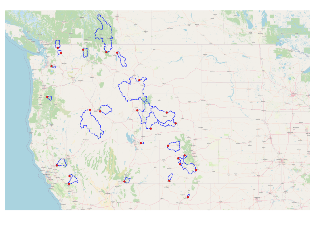
DrivenData is currently (spring 2024) hosting another Bureau of Reclamation competition to predict water supply volumes in 26 basins scattered across the Western US (see Figure 1). Specifically, the goal is to predict total stream flow at the basin outlet over several months in the spring and summer. This is critical information used by water managers and water users to plan activities like irrigation and hydroelectric power generation. The spring and summer timeframe is important because, in the Western US, a majority of the surface water supply is generated by snowmelt (Fleming et al., 2021). So, most of the flow volume occurs in the spring during snowmelt and is often stored in reservoirs for later use.
As was the case with the 2022 snow competition, I find that these competitions require the perfect combination of hydrology, mathematics, data engineering, and computing skills for the expertise that I am cultivating. So, I couldn’t resist getting involved. The prize money is also substantial, but I don’t consider myself to be competitive at that level yet.
There are two aspects of this water supply competition that make it particularly challenging (at least from my perspective). The first is a requirement to generate multiple forecasts throughout the winter and spring. Forecasts begin as early as January 1st and earlier forecasts will necessarily have more uncertainty than later forecasts because parameters like peak snowpack are not yet known. Predicting the climate months in advance is also very difficult. Another requirement is to issue “quantile” forecasts which include an estimate of uncertainty in the prediction. For example, instead of predicting a specific flow volume, the forecast is given such that the volume will be above a certain amount (“90% chance total flow volume exceeds 10000 acre-feet”).
Natural Resource Conservation Service
Forecasting spring flow volumes has a long history, and, in the US, has primarily been the domain of the Natural Resource Conservation Service (NRCS). The NRCS, whose primary mission is focused on agriculture, seems like an unusual candidate for snow pack monitoring and runoff forecasting, especially given that the USGS is typically in charge of making the flow measurements. However, the need for flow forecasting was driven in part by water users including irrigators. This led the predecessor of the NRCS, the “Bureau of Agricultural Engineering” to take the lead in establishing a snow survey program in the early 20th century (Helms et al., 2008).
Some of the earliest snow pack measurements in the Western US began in the late 1800’s in California. As early as the 1930’s, there was a need for flow forecasting and the general approach was to relate snow in a given location to flow at a given location. Today, the NRCS uses the “VIPER” system which utilizes watershed specific linear regressions, but is highly flexible in terms of input types and data quantity (see NRCS Technical Note). Surprisingly, VIPER is Excel based rather than implemented in a programming language. I am guessing Excel is used because the analysts are more familiar with Excel than a scripting language like Python, but implementing it must have been painful.
| Example VIPER Inputs |
|---|
| Peak SWE multiple station |
| Season start SWE multiple stations |
| Climate index like ENSO |
| Antecedent streamflow |
| Precipitation from multiple stations |
VIPER makes flow volume predictions via either “principle component analysis” or “Z-score regression”. While both of these methods utilize linear regression, in the case of Z-score regression, the various inputs are combined into a composite variable before computing the linear regression. Principle Components Analysis, on the other hand, is used to eliminate correlations between input variables. For example, two different Snotel stations in the same basin are likely to be highly correlated. These correlations can cause problems in the linear regression because each variable is conveying duplicate information to some extent. Ideally, each input should be explaining the output variance in a different way.
In addition to the regression methods used, VIPER also optimizes the inputs for a given watershed. Flow volume in one watershed might depend on peak snowpack where in another basin flow might depend on a combination of snow and antecedent flow.
Watershed Hydrology
It seems that many machine learning models, including models that win competitions, are essentially black boxes. Large amounts of training data are crammed into the model, and it automatically figures out the relationships between inputs and outputs. There are various approaches for interpreting what data is most important after the fact, but the main challenge is to identify what modeling approach works best and how to tune the model correctly. I haven’t yet reached that level of familiarity with all the different machine learning techniques, so I try to leverage my knowledge of hydrology to give myself some sort of competitive advantage.
A simple model of basin hydrology, created using conservation of mass, is quite useful for getting a better understanding of the essential data needed for predicting flow volumes. Hydrologic basins, also known as “catchments” or watersheds are defined as areas upstream of a location (the outlet) on the landscape, such that all the precipitation falling on that area could theoretically follow a surface flow path to the outlet (Hornberger et al., 1998). The perimeters of the 26 basins in this competition are already delineated (figure 1) with respect to the location where flow volume is to be predicted.
For each basin, over the course of the flow season: Inputs – Outputs = Change in Basin Storage
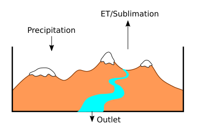
Inputs are precipitation in the form of rain or snow. By definition, there are no surface flows of water into the basin. It is assumed that groundwater is also not moving in or out of the basin perimeter (which might not be true in some situations). Outputs include evapotranspiration (ET), sublimation, and, of course, streamflow at the basin outlet, which is the target of the competition. Water can be stored within the basin as snow, surface water, or groundwater. After all of the basin inputs and outputs are accounted for, we can solve for the target variable “flow volume”.
Outlet flow volume = Rain + Snow – ET – Sublimation – Δ(snowpack, groundwater, surface water) [EQ1]
If all the variables in equation 1 were known, the flow volume could simply be calculated. However, some, like ET and sublimation, are tricky to measure let alone predict at a future time period. Estimating the change in storage is also tricky because movement of water between the different types of storage, especially snowmelt to groundwater, doesn’t necessarily change the overall amount of water in the basin. Nonetheless, equation 1 provides a framework for determining what input data I should focus on and how the different datasets relate to one another.
Linear Modeling
My approach to these DrivenData competitions has basically been to start as simply as possible and add on complexity depending on performance and available time. Unfortunately, I only seem to have time to do the bare minimum. On the other hand, I continue to be surprised by how good a job a simple model can do. In this case, I just use linear regression to relate snowpack (SWE) to river flows. That is essentially what the NRCS already does, but instead of using Snotel measurements as direct inputs, I utilize the NOAA snow model SNODAS to estimate total basin SWE. While I found problems with SNODAS in prior projects, it still seemed like a good option given that it has output covering each of the basins, including one basin extending into Canada. The total amount of SWE in a basin provides a more direct relationship between snow and river flow as compared to SWE at one or two locations, and eliminates the need for Principle Component Analysis. Considering only snow is a major simplification of equation 1, but it is a reasonable starting point assuming snowpack is the dominant factor.
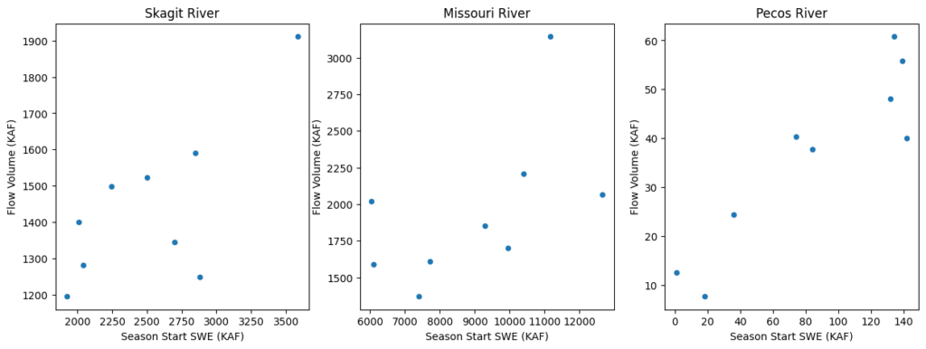
My machine learning model actually consists of two linear regression models. The first regression relates total SWE in the basin at the start of the flow season to total flow volume for each basin. Figure 3 shows the relationship between Season Start SWE and total flow volume for three different basins in the competition. Despite the fact that there is Snotel data going back to the 1970’s (older?), SNODAS has only been available since 2005. So, only 9 data point are available in each watershed for determining the regression (odd years are withheld for testing). This is a major weakness to my approach.
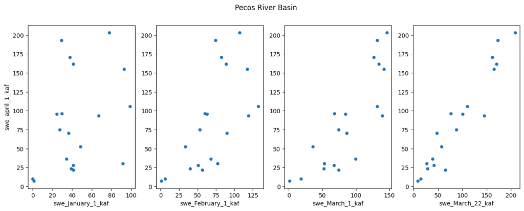
A second linear regression is needed to predict the start of season total SWE from snowpack on a given date. I create a new regression for each basin and forecast date (figure 4). As can be seen in figure 4, earlier forecasts have more uncertainty because it is hard to predict based on historical data whether a low snowpack will recover (or vice versa) looking ahead from January. Luckily, there is enough inertia in the system that deeper snowpacks early in the year often lead to big snowpacks by the start of flow season.
Although I was able to submit model predictions to the competition using just snow as an input, I had some extra time left to try and improve the model. The quickest option appeared to be to incorporate “antecedent flow” into the model. Antecedent flow is the flow volume at the outlet over some period of time prior to the flow season, such as flow from January to April. The competition conveniently provided this data, eliminating the need for any data engineering and lowering the implementation time. However, it wasn’t clear exactly how antecedent flow fit into my hydrology model. It seems like it might provide some indication of the state of the groundwater, but not in any direct way.
I ended up simply adding it as another regression parameter in the model such that total flow season volume is a function of both snowpack and antecedent flow. Once again, I predict future antecedent flow as a linear function of flow on a given date. I had high hopes that the improved model would lead to better results, but it didn’t turn out that way.
Implementation
All the steps required for both data engineering and regression modeling were completed using Python and the code is available on Github. Data engineering involves creating model inputs from whatever raw data sources are available. Often data needs to be cleaned, re-organized, or transformed prior to use. For the most part, all my coding is done in a Jupyter Notebook which hopefully makes it easier to follow for anyone interested, or just as likely, my future self.
SNODAS data is automatically retrieved from NOAA, but many steps are required to use it in the model. Once SNODAS model data for a particular date is downloaded, it must be unzipped and the raw contents converted into a GeoTiff for analysis. For this, I use the RasterIO package which, in turn, uses GDAL to make the conversion. Another library RasterStats is used to calculate total snow water equivalent within a given basin. This is repeated for all the dates needed for training the model (~ 300).
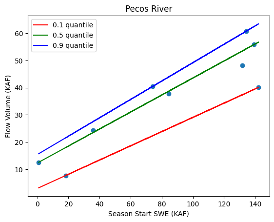
Once all the training data has been extracted, I can begin computing the various linear regressions that make up the model. Rather than computing a single seasonal flow prediction at each site on the forecast dates, the competition requires “quantile predictions”. Quantile regression still produces a linear function relating input (such as snow) to output (flow volume), however, the regression line for a given quantile will be shifted and/or rotated to form upper or lower bounds on the training data. Figure 5 shows the quantile regression lines used in the Pecos River Basin. Unlike regular least squares linear regression, there is no analytical solution for quantile regression. I used the SciKit Learn Python Package which includes a quantile regression solver. It uses a SciPy optimization algorithm to find a solution.
Results
The competition provides flow data from each of the basins going all the way back to the 1910s for training. Ten odd numbered years of historical flow data are held back for testing. There are about 28 forecast dates per site in each test year and three predictions, corresponding to the three quantiles, are made on each date. This gives a total of about 21,000 predictions that are submitted to the competition for evaluation. Each submission is evaluated using the test data and a “pinball” evaluation metric (see https://scikit-learn.org/stable/modules/model_evaluation.html#pinball-loss).
Given the simplicity of my approach, I was surprised to find that my first submission ranked 23rd out of 509. The unexpectedly good performance of my model inspired me to try some simple improvements and I went ahead and implemented the model with antecedent flow as another regressor. Unfortunately, adding antecedent flow to the model actually decreased the performance, and I am not sure why.
Conclusion
This is the second machine learning competition I have participated in, and I continue to be surprised by how well I do without relying on sophisticated techniques like neural networks. Having more time to build a model would likely improve my ranking, however, being part of the right team would probably be even more impactful. Unfortunately, I have had trouble finding other who are interested in joining me. Regardless, I suspect breaking into the top ten probably does require a lot more sophistication, so it will be interesting to assess the competition winners later this year.
References
Fleming, S. W., Garen, D. C., Goodbody, A. G., McCarthy, C. S., & Landers, L. C. (2021). Assessing the new Natural Resources Conservation Service water supply forecast model for the American West: A challenging test of explainable, automated, ensemble artificial intelligence. Journal of Hydrology, 602, 126782.
Helms, D., Phillips, S. E., & Reich, P. F. (2008). The history of snow survey and water supply forecasting: Interviews with US Department of Agriculture pioneers (No. 8). US Department of Agriculture, Natural Resources Conservation Service, Resource Economics and Social Sciences Division.
Hornberger, G. M., Wiberg, P. L., Raffensperger, J. P., & D’Odorico, P. (1998). Elements of physical hydrology. JHU Press.
NRCS Technical Note, Statistical Techniques Used in the VIPER Water Supply Forecasting Software, Accessed from https://www.nrcs.usda.gov/resources/data-and-reports/publications-of-the-national-water-and-climate-center.