
In my last blog post, I tried to answer the question:
How has snowfall at Sandia Peak Ski Area changed over the years?
Ultimately, I want to know how climate change is affecting the future of skiing in the Sandias and to develop some sense of what weather patterns are associated with particularly good or bad years. With that in mind, I focused my initial research on assessing daily SWE values at the Ski Area. Unlike daily snowfall or total seasonal snowfall, daily SWE represents the actual amount of snow on the ground, including the effects of melting, sublimation, and redistribution from wind. Furthermore, since SWE is fundamentally a measure of water quantity, this analysis not only describes the overall quality of the snow for skiing, it is also equally useful from a hydrologic perspective.
The Sandias are lacking direct measurements of daily SWE values. So, I utilized a reconstruction of both SWE and snow depth from a model developed by the University of Arizona called SWANN. (Note that in the prior blog post I referred to the dataset as the “4km snow grid” because my only source for the data at that time, the NSIDC, didn’t have a specific name for the dataset). While the methodology for developing the model output seemed robust (Broxton et al., 2016), it was still an open question as to how accurate the model was in the Sandias specifically. Indeed, a reasonable criticism was that the dataset suffers from problematic model inputs. Specifically, radar based estimates of precipitation over the Sandias are bias low because the radar beam located west of the area is blocked by the west face of the Sandias causing a radar “blind spot” right where the ski area is located (more on this below). To better assess the performance of SWANN at Sandia Peak Ski Area, I decided to make some comparisons with actual field data, as well as, a second snow pack model developed by the National Weather Service called SNODAS.
One surefire way of getting direct measurements from the field is to do them yourself. So, I made several measurements in March and April of this year (2023) at the ski area using my own “DIY” approach. I also collaborated with Kerry Jones (@peakwx) and Brian Guyer, two experienced meteorologists. Kerry has a number of historical images of snow along the Crest Road (NM 536) that I used to get a semi-quantitative estimate of snow depth. Finally, it turns out there is a relatively new research weather station in the Sandias near the Ski Area that I wasn’t aware of until just this last spring. The station was recently upgraded, and it has been measuring snow depth since fall of 2022. None of these comparison datasets extend back in time beyond about 2005, but they are nonetheless a good starting point for evaluating SWANN in the Sandias from a wide variety of perspectives.
Field Photos
Given the right context and location, photographs of snow in the Sandias, are a useful comparison to snow pack models. Lacking a ruler of some sort in the picture, the precise depth of snow may not be easy to extract from the image. However, relative snow depths from pictures taken at the same location can be assessed based on static features in the landscape, like trees.
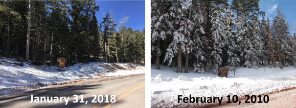
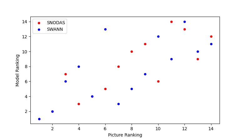
Starting in 2009, Kerry Jones and another meteorologist, Brent Wachter, began taking photographs of the snow adjacent to the road near the crest (see figure 2). A few images are captured each year around early February, and most feature a trailhead sign, giving a fixed reference from which to compare two different years. I ranked each of Kerry’s photographs from lowest snow to highest (1 to 14) and then compared snow depths extracted from the SWANN and SNODAS models for the same date (figure 3).
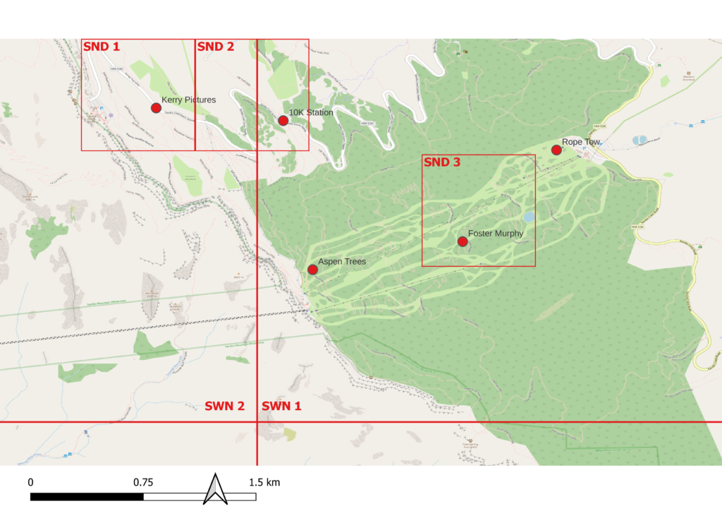
Note that the SNODAS snow depths are from the SNODAS grid cell encompassing the picture location (labeled SND1 in figure 1). However, the SWANN snow depths are from the grid cell located just east of the picture location (labeled SWN1 in figure 1). The SWANN grid cell encompassing the picture location (SWN2) includes the high relief topography of the west face of the Sandias and is likely to be less representative of snow conditions at the picture location than the grid cell to the east.
While the picture ranking and snow model ranking have a fair amount of scatter, there is still a good correlation between the two indicating the models are faithfully representing good and bad years. Much of the scatter is likely due to the difficulty in ranking pictures with moderate levels of snowfall. In contrast to figure 2, where it is easy to distinguish which date has deeper snow, most of the comparisons between pictures were a bit subjective.
Field Data Comparisons
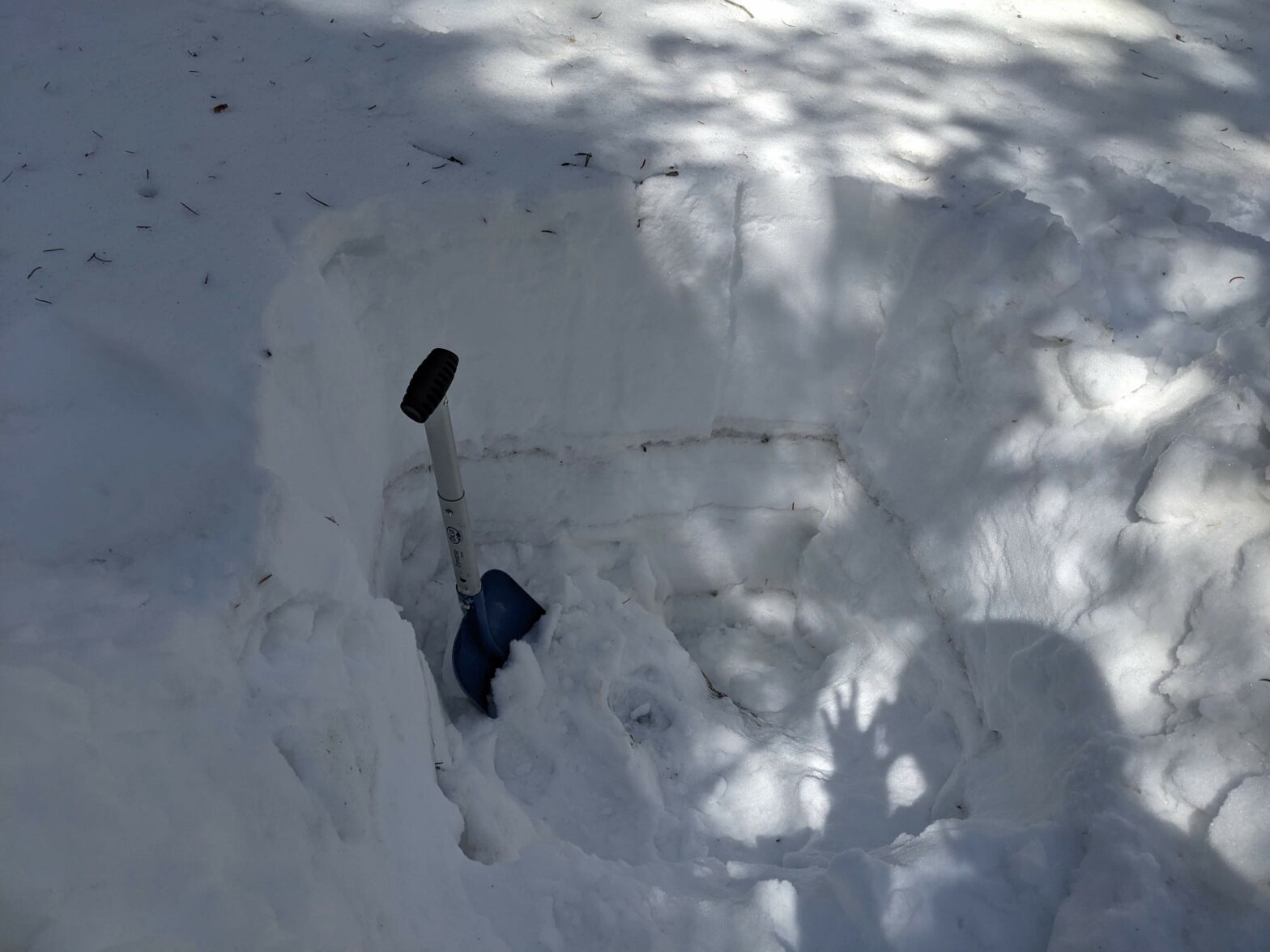
Throughout March and April of this year (2023), I visited the ski area 5 times and collected both snow depth and SWE data. I chose three different sites: near the base, near the top, and mid-mountain (see figure 1) in order to get a sense for how the snow pack varies with elevation. Given the amount of time and resources available, I limited SWE measurements to just the mid-mountain site (table 1).
| Date | Site | Snow Depth (in) | SWE (in) |
|---|---|---|---|
| 3/3/2023 | Rope Tow | 30.5 | |
| Foster Murphy | 32.5 | 8.5 | |
| Aspen | 29.5 | ||
| 3/23/2023 | Rope Tow | 38 | |
| Foster Murphy | 53 | 14.9 | |
| Aspen | 59 | ||
| 4/11/2023 | Rope Tow | 12 | |
| Foster Murphy | 43 | 15.1 |
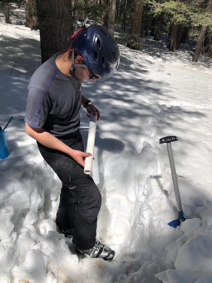
SWE is typically measured using a stainless steel tube and a scale. My methodology was less refined, but sufficient for this analysis. I simply used a section of pvc pipe to extract a snow core that I put in a bottle and brought home for melting. I couldn’t extract the whole core at once, and each successive section of snow, no doubt, introduced error. Furthermore, I only made one measurement per site visit, so there is no information about local spatial variability. Nonetheless, my sense is that there is enough precision in my field measurements for general comparisons with other sites and to assess SWANN and SNODAS model performance.
I wasn’t the only one making snow measurements in the Sandias this past winter. Adrian Marziliano is a PhD candidate at UNM working with Professor Ryan Web. His research focuses on satellite-based snow measurements with field work in the San Juan Mountains of Colorado. Adrian has also been working in the Sandias maintaining a weather station near the 10K trailhead. This station has recently (fall 2022) been equipped with a snow depth sensor. Additionally, Adrian has been conducting manual snow depth measurements on a snow course adjacent to the station. Adrian was kind enough to share several snow depth and SWE measurements from the 2021/2022 and 2022/2023 seasons, as well as, 15 minute snow depth data from the 10K station from last season. As of this writing, the station data more recent than February 2023 has yet to be collected.
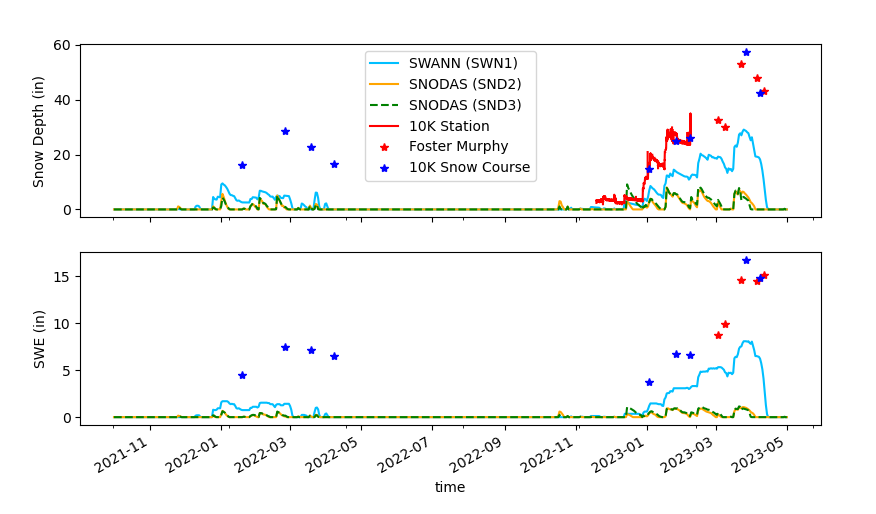
Figures 4 shows depth and SWE comparisons between both models and field measurements. It is important to note that the field measurements and model locations do not all overlap (see figure 1). For example, my “Foster Murphy” field site is approximately 1 mile from the 10K station, but is still within the SWANN SWN1 grid cell. Despite these differences, I think the distances and topography of the area are such that it is still reasonable to compare the different datasets to assess model performance.
There are several interesting takeaways from the comparisons. As might be expected, Adrian’s depth measurements match those measured by the snow depth sensor at the 10K station. Furthermore, the high resolution station data shows changes in depth that are very similar to the SWANN data and, to a lesser extent, the SNODAS data. The 2021/2022 SWANN data is arguably less similar to Adrian’s field measurements than in 2022/2023, but it is still more representative than SNODAS.
My field measurements of both depth and SWE (Foster Murphy) are broadly similar to those measured by Adrian (10K Snow Course). This supports the idea that the snowpack variability across this one-mile area is low, which gives me more confidence in comparing point measurements to larger scale model grids. Another takeaway from the comparisons is that the SWANN model appears to be much closer to the field measurements than SNODAS. Nonetheless, SWANN underestimates snow at both field sites, and this isn’t too surprising because, at the SWANN grid scale (~4 km), there is a gradient in snow accumulation (see Table 1: 4/11/2023) which SWANN is averaging over. It might be possible to downscale the SWANN output using snow pack elevation gradients, but I didn’t feel that was needed at this time.
Model Comparisons
Given the substantial differences between SWANN and SNODAS models, I decided it would be useful to investigate what might be the cause. As detailed in my previous blog post, SWANN is a 4km gridded snow model built by the University of Arizona. In contrast, SNODAS is a 1km snow model built and run by NOAA’s NOHRSC. It covers the entire continental US and parts of Canada, runs on an hourly time step and produces a wide variety of outputs including SWE and snow depth, as well as, more unique outputs like snow temperature (see NOHRSC, 2004). SNODAS utilizes large amounts of real world data like SNOTEL measurements and meteorological observations to run a multi-layered snow model: SNTHERM (Barrett, 2003). The snow model simulates relevant snow pack processes like melt water infiltration. Interestingly, forecasters with NOHRSC actively participate in SNODAS operation by making corrections to the model based on model performance with respect to field data.
When comparing the model output to point measurements (figure 4), I generally compared the field measurement to the closest model grid cell (see figure 1). However, when comparing the models for longer time periods, I figured it would be best to re-sample the 1km SNODAS data to the 4 km grid size of SWANN. That way if there happened to be some local anomaly at the 1km scale it wouldn’t bias the comparison. To perform the resampling, I took a simple approach of averaging all the 1km SNODAS grid cell values inside the overlapping 4km SWANN grid cell.
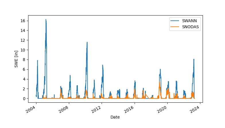
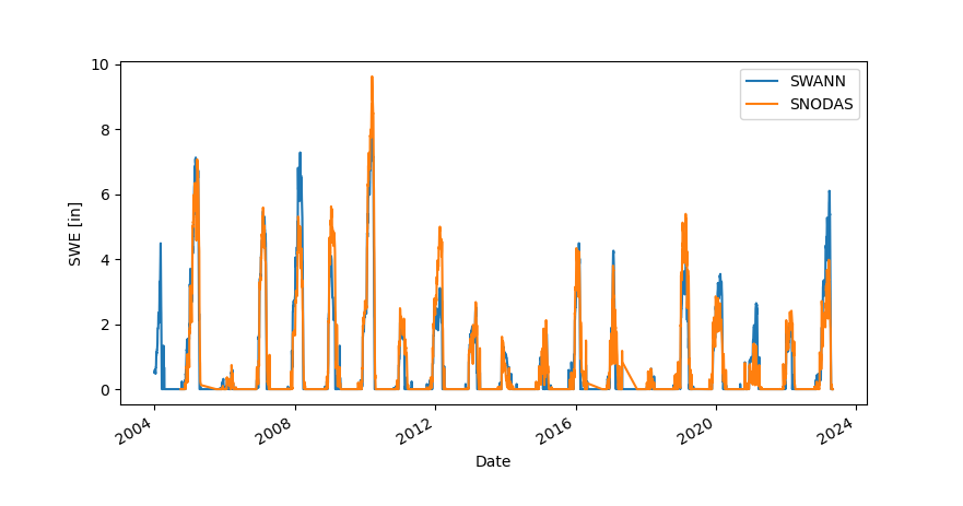
As was the case with the point comparisons, the SNODAS data is much lower than the SWANN data for both SWE and snow depth (figure 5). Some years the difference is glaring, with SNODAS showing no snow on the ground while SWANN is showing 16 inches SWE. Overall the mean absolute difference in SWE is 1.76 in with a standard deviation of 2.54 in (summertime values removed). For comparison, Broxton et al. 2016 show a mean absolute difference of 2.75 in SWE comparing SNODAS to SWANN in the northern Rockies, but that analysis looked at spatial differences not differences through time. I browsed the literature to see if there were any known geographical biases in SNODAS. In general, SNODAS can be difficult to independently evaluate because much of the field data commonly used to evaluate snow models gets assimilated into SNODAS. Hedrick et al. 2015 assessed SNODAS performance in northern Colorado using both lidar and in situ field measurements. Their findings also focused on spatial differences and were mostly consistent with prior work that indicated SNODAS under predicted snow depth in alpine environments due to the influence of trees and complex topography.
There seems to be something particular to the Sandias that is influencing SNODAS, and I suspect it is the very thing that originally inspired this follow-up investigation: radar beam blockage. Radar is a focused beam of radio or microwaves with a width of about 1 degree rotating in a circle to scan a 360 degree view for about 120 miles (see https://www.noaa.gov/jetstream/vcp_max). As the radar rotates, the beam sweeps through predefined horizontal and vertical coverage patterns to obtain a volumetric analysis of the atmosphere. If the position of the radar transmitter is such that the beam encounters topography during it’s scan, it is effectively blocked from viewing any area behind the obstacle as a function of the beam angle and distance from the transmitter.
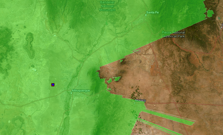
The Sandias are situated such that radar from KABX is blocked for a region almost directly over the ski area. Figure 6 shows radar coverage at 3000 feet above ground level in green. There is a clear gap in coverage behind (east of) the Sandias (https://www.ncei.noaa.gov/maps/radar/). I couldn’t find a coverage map for heights below 3000 feet, but it is clear the beam won’t be “seeing” the back side of the Sandias. This is especially problematic for winter storms and shallow convection (Kerry Jones per comm.) Not only is radar important for identifying where precipitation is taking place, it is also used to estimate the amount of precipitation that has fallen. Theses total precipitation estimates are integrated into meteorological models like the HRRR which is then used by SNODAS for determining snow pack (https://www.nohrsc.noaa.gov/technology/). In contrast to SNODAS, SWANN doesn’t use radar for precipitation estimates. Instead precipitation is provided by PRISM which essentially does sophisticated interpolation of station measurements (Daly and Bryant, 2013).
As a final check, I decided to compare SNODAS (re-sampled) and SWANN near Pajarito Ski Area in the Jemez mountains, just west of Los Alamos. Here the radar beam is not blocked by terrain, and the aspect and terrain is somewhat similar to that of the Sandias. Clearly the difference between the two model snow depths is much smaller (figure 7) at this site than in the Sandias.
Conclusion
Overall, the combination of field and model comparisons gives me more confidence in the SWANN reconstruction of Sandia’s snow history. I still wish we could look back farther in time to see how much snow there was in the 1930’s when Sandia Peak Ski Area was first established. Nonetheless, the 40 year record has a lot of potential to explain what causes snowy or dry winters and what impacts climate change is having on the mountain.
References
Barrett, A. 2003. National Operational Hydrologic Remote Sensing Center SNOw Data
Assimilation System (SNODAS) Products at NSIDC. NSIDC Special Report 11. Boulder,
CO, USA: National Snow and Ice Data Center. Digital media.
Broxton, P. D., N. Dawson, and X. Zeng, 2016, Linking snowfall and snow accumulation to generate spatial maps of SWE and snow depth, Earth and Space Science, 3, 246–256, doi:10.1002/2016EA000174.
Daly, C. and Bryant, K., 2013, The PRISM Climate and Weather System – An Introduction, downloaded from https://prism.oregonstate.edu/documents/PRISM_history_jun2013.pdf.
Hedrick, A., Marshall, H.P., Winstral, A., Elder, K., Yueh, S. and Cline, D., 2015. Independent evaluation of the SNODAS snow depth product using regional-scale lidar-derived measurements. The Cryosphere, 9(1), pp.13-23.
National Operational Hydrologic Remote Sensing Center. 2004. Snow Data Assimilation System
(SNODAS) Data Products at NSIDC, Version 1. Boulder, Colorado USA.
NSIDC: National Snow and Ice Data Center. https://doi.org/10.7265/N5TB14TC.