
Part 1: Competition Overview
Late last December I ran across a machine learning competition hosted by Driven Data. The goal of the competition is to predict snow water equivalent at high spatial resolution across the western US. I had never before thought of participating in a machine learning competition, although I had heard of the idea via another platform, Kaggle. However, a machine learning competition involving snow is more up my alley, as I have both professional and personal experience with snow science. Furthermore, I had been wanting to enhance my familiarity with machine learning techniques. I decided to give it a shot.
The competition is funded by the US Bureau of Reclamation and includes some significant prizes including $150K for first place. The Bureau of Reclamation manages dams and water systems across the Western US, and works closely with the Natural Resources Conservation Service who maintain the Snotel network, a nationwide system of snow monitoring stations. One use of the Snotel Network is to predict stream flow during Spring snow melt which is used for reservoir management and irrigation. With a prize money totaling $500K, it is clear that this sort of analysis is highly valued by water managers and users.
Winning the competition is definitely challenging. SWE predictions must be submitted for thousands of 1km x 1km grid cells located across the Western US (figure 1), with high density clusters of cells located in the Rocky Mountains and Sierra Nevada. Each prediction corresponds to a particular date, and several weeks worth of predictions are made for each grid cell. The competition is divided into two stages: “development” and “evaluation”. In the development stage, each competitor is tasked with developing a model that makes SWE predictions at a subset of grid cells using some combination of the following as inputs:
- Historical Snotel data (provided by the competition)
- SWE observations in a subset of grid cells (provided by the competition)
- Other relevant publicly available data such as satellite observations and weather models
The submitted predictions are evaluated against known values (not available to the competitors). No prizes are awarded, but competitors can evaluate how their submissions compare using the root mean square error (RMSE) of the predictions vs the actual values. During the evaluation stage, finalized models are submitted to the competition and predictions are made in real time using live data. These predictions are then evaluated against actual field measurements made throughout the Spring. The best performing model during the real time data competition wins the prize.
Despite my excitement for the challenge, my current life situation limited the amount of time I would be able to spend competing. I looked into forming a team, but my network didn’t yield any takers (contact me if you are interested in this kind of thing). I decided it was best to pursue just the development stage of the competition and see what ranking I might achieve using whatever simple model I could create. This path eliminated the possibility of prizes, but I could still evaluate my performance.
Snow Water Equivalent
Snow water equivalent is the amount of water you would get if you melted the snow at some location. This is more useful than snow depth itself, especially for water resources, because snow consists of layers with different densities. The densities in each layer are a function of the atmospheric conditions when snow formed, as well as, changes that take place after the snow has fallen. Two areas with the same snow depth may have very different amounts of equivalent water.
To manually measure SWE one must go out in the field and collect a column of snow, then weigh it to get the average density. With a known density and volume, the measurement can then be converted to SWE. For example, here in New Mexico, the snow pack is thin, typically less than 3 feet deep. An average density for a mountain snow pack might be around 0.3 g/cm3 (Sturm et al., 2010) (ice ~ 0.9 g/cm3, water = 1 g/cm3). To calculate SWE for a snow depth of 24 inches (~60cm):
Mass of snow in rectangular volume: 0.3 g/cm3 * 60cm * 1cm2 (arbitrary area) = 18 g
Equivalent volume of water: 18 g divided by 1 g/cm3 = 18 cm3
SWE: 18 cm3 / 1cm2 (arbitrary area) = 18cm ~ 7 inches
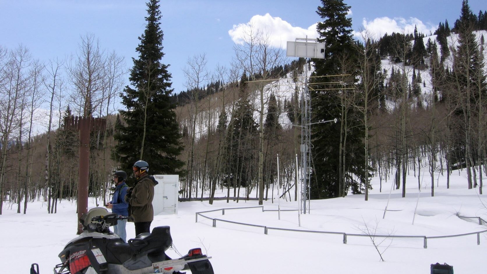
Snotel is a network of monitoring stations managed by the NRCS that automatically measures SWE (figure 2). To do this, the stations use a “snow pillow” which is basically a fluid filled bag positioned under the snow. Pressure on the bag determines the weight of the snow and other sensors determine the depth. SWE is calculated from these raw measurements and transmitted via satellite back to a database. The Snotel measurements are key inputs for predicting high resolution SWE, but in many places the stations are few and far between.
Competition Data Exploration
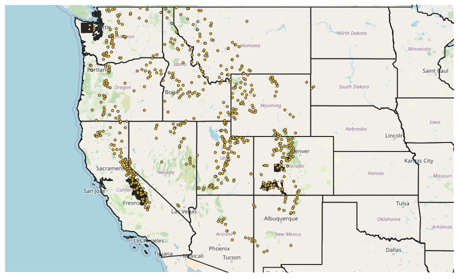
I used QGIS for some initial data exploration as well as more in depth analysis (more details given in a future blog post). Figure 2 shows the grid cells located in southwestern Colorado. In general, cells are clustered over mountain ranges, as might be expected, but the cells are not a uniform grid. This may be due to the availability of field data or perhaps the cells in the competition are meant to be distributed somewhat randomly across different areas of focus. Snotel sites are also shown in Figure 2 (orange dots) and are much more sparse than the grid cells.
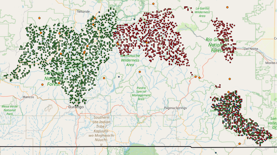
Of the 11,000 grid cells, a subset of grid cell locations have data that can be used for model training. Another subset has no training data, but are areas where predictions are made for submission. Some of the cells are both training and submission cells. I identified which cells were of the different types using a Python script and then displayed the cell type on the map using different colors: green = training, red = submission, blue = both. In some places, training cells are located in separate clusters from submission cells, while in others there are cells of each type clustered together (see figure 2). Again, it is unclear why the competition is structured in this way, but the takeaway seems to be that any model will need to applied to a wide variety of latitudes, elevations, aspects, and mountain ranges.
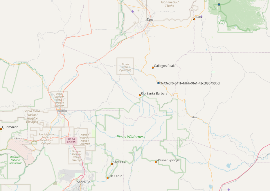
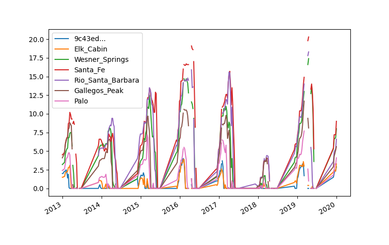
In New Mexico, cells are fewer and much farther apart and there are less Snotel stations. For example, one of the grid cells in western NM doesn’t even have a Snotel within 300 km of the cell location. However, there is a NM grid cell (ID 9c43…) in the Sangre de Cristo mountains between Santa Fe and Taos located near 6 different Snotel sites (figure 3). Since I am familiar with this area, I thought it would be a good location to get a better sense for how the training data compares to the Snotel data. I located all the Snotel sites within 50km of the grid cell and plotted a time series of both the grid cell and Snotel data (figure 4). The grid cell data is most similar to the “Elk Cabin” Snotel site which is actually farther away than several other sites. The closest site, Gallegos Peak, typically has much more SWE than the grid cell. This indicates elevation is playing a more significant role in SWE values than location.
My Approach
The importance of snow in the hydrologic cycle, especially in the arid west, means estimation of SWE is an important area of academic and government research. Rather than try to come up with an approach for predicting SWE from scratch, I performed a literature search to see what machine learning techniques others had used. As might be expected, there is a wealth of publications on the topic, and my review was brief given my time constraints. Furthermore, I stopped looking for new articles when I found a method, detailed by Fassnacht et al. 2003, that was straightforward enough for me to implement in a short amount of time.
I found three general approaches to estimating SWE from the smattering of articles I reviewed:
- SWE Reconstruction
- SWE from density modeling
- SWE from interpolation
I found the first approach, SWE reconstruction, to be quite clever, and it is described thoroughly by Rittger et al. 2016. This method works backwards using satellite imagery and a snow melt model. Satellite data is frequently used to determine snow cover extent, but estimation of SWE directly from satellites is still a problem (Schneider and Molotch, 2016). A melt model predicts how much snow will melt given inputs like temperature and solar radiation. The satellite determines the date the snow melts completely (SWE = 0) at a given point and the melt model determines how much total melt took place, so together a maximum value of SWE can be determined (Rittger et al. 2016, Bair et al., 2016). Unfortunately, this method cannot be utilized to predict SWE in real time.
The second method calculates SWE by first estimating the snow density at a location. The density must still be combined with snow depth in order to calculate SWE (see SWE overview), but often times snow depth is much easier to measure over a broad region than other snow parameters. For example, the Airborne Snow Observatory is a NASA mission that uses planes to collect snow depth data using LIDAR. LIDAR uses lasers to create very high spatial resolution depth measurements over a large area. However, these depth measurements cannot be converted to SWE without density. Jonas et al. 2009 predict snow density using a regression on season, depth, elevation, and other factors. Similarly, Sturm et al. 2010 predicts snow density based on climate classifications such as “tundra”, “prairie”, and “alpine”. Density based methods could be used in real time so long as snow depths are also collected in real time.
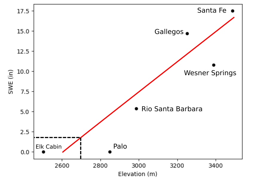
The last approach I found for estimating SWE is to use some form of interpolation (Schneider and Molotch, 2016, Fassnacht et al. 2003). With interpolation, high spatial resolution SWE values are calculated from sparse SWE measurements (such as Snotel measurements). For example, Bair et al. 2016 use 3D bilinear interpolation as one of several methods they compared. Fassnacht et al. 2003 also compare some different interpolation methods and detail the “hypsometric method”. Hypsometric is a term related to the measurement of heights, and this method utilizes Snotel measurements to create a regression against elevation. This regression is then used to predict the SWE at different elevations in a given area. For example, figure 5 shows a plot of SWE values as a function of elevation from the six Snotel sites near Santa Fe, NM on a randomly chosen date in the dataset (2016-04-05). A regression is fit to the points and a predicted value of SWE is obtained from the elevation of the grid cell. Since the grid cell elevation is ~2700m the predicted SWE is about 2 inches. This method, and most other interpolation methods, can be used in real time if the input values, such as Snotel SWE measurements, are collected in real time.
Given the simplicity and support in the literature for the hypsometric method, I decided to give it a try. In Part 2 of this blog post, I describe how I implemented the approach and the results after I submitted my predictions to the competition. I did much better than I thought I would!
References
Bair, E. H., Rittger, K., Davis, R. E., Painter, T. H., & Dozier, J. (2016). Validating reconstruction of snow water equivalent in California’s Sierra Nevada using measurements from the NASA Airborne Snow Observatory. Water Resources Research, 52(11), 8437-8460.
Fassnacht, S. R., Dressler, K. A., & Bales, R. C. (2003). Snow water equivalent interpolation for the Colorado River Basin from snow telemetry (SNOTEL) data. Water Resources Research, 39(8).
Jonas, T., Marty, C., & Magnusson, J. (2009). Estimating the snow water equivalent from snow depth measurements in the Swiss Alps. Journal of Hydrology, 378(1-2), 161-167.
Rittger, K., Bair, E. H., Kahl, A., & Dozier, J. (2016). Spatial estimates of snow water equivalent from reconstruction. Advances in water resources, 94, 345-363.
Schneider, D., & Molotch, N. P. (2016). Real‐time estimation of snow water equivalent in the U pper C olorado R iver B asin using MODIS‐based SWE Reconstructions and SNOTEL data. Water resources research, 52(10), 7892-7910.
Sturm, M., Taras, B., Liston, G. E., Derksen, C., Jonas, T., & Lea, J. (2010). Estimating snow water equivalent using snow depth data and climate classes. Journal of Hydrometeorology, 11(6), 1380-1394.