
Part 1: Quality Control Background
Overview
This is the first of a 2 part series on automated quality control of environmental data. This part gives an overview of quality control methods and the second part (under development) details how I used Python to create a demonstration API (api.crceanalytics.com) that performs automated QC on uploaded air temperature data.
Environmental Data Quality Control
Data is always going to need some sort of quality control after it is collected. This is especially true of environmental data collected from autonomous sensors placed in challenging environments. Sensors often break or experience electrical problems that lead to gaps in data and/or anomalous readings. Furthermore, bad data may also result from calibration or maintenance performed while the sensor is operating. Preventative maintenance and ongoing data monitoring, practices known as quality assurance (Campbell et al., 2013), help to reduce that amount of problematic data collected. However, as sensor technology gets cheaper, much more data is collected and manual methods for identifying suspicious and bad data becomes increasingly difficult and subjective (Jones et al., 2018). Automation of data quality control is going to be increasing important for ensuring high quality environmental data.
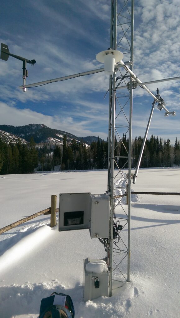
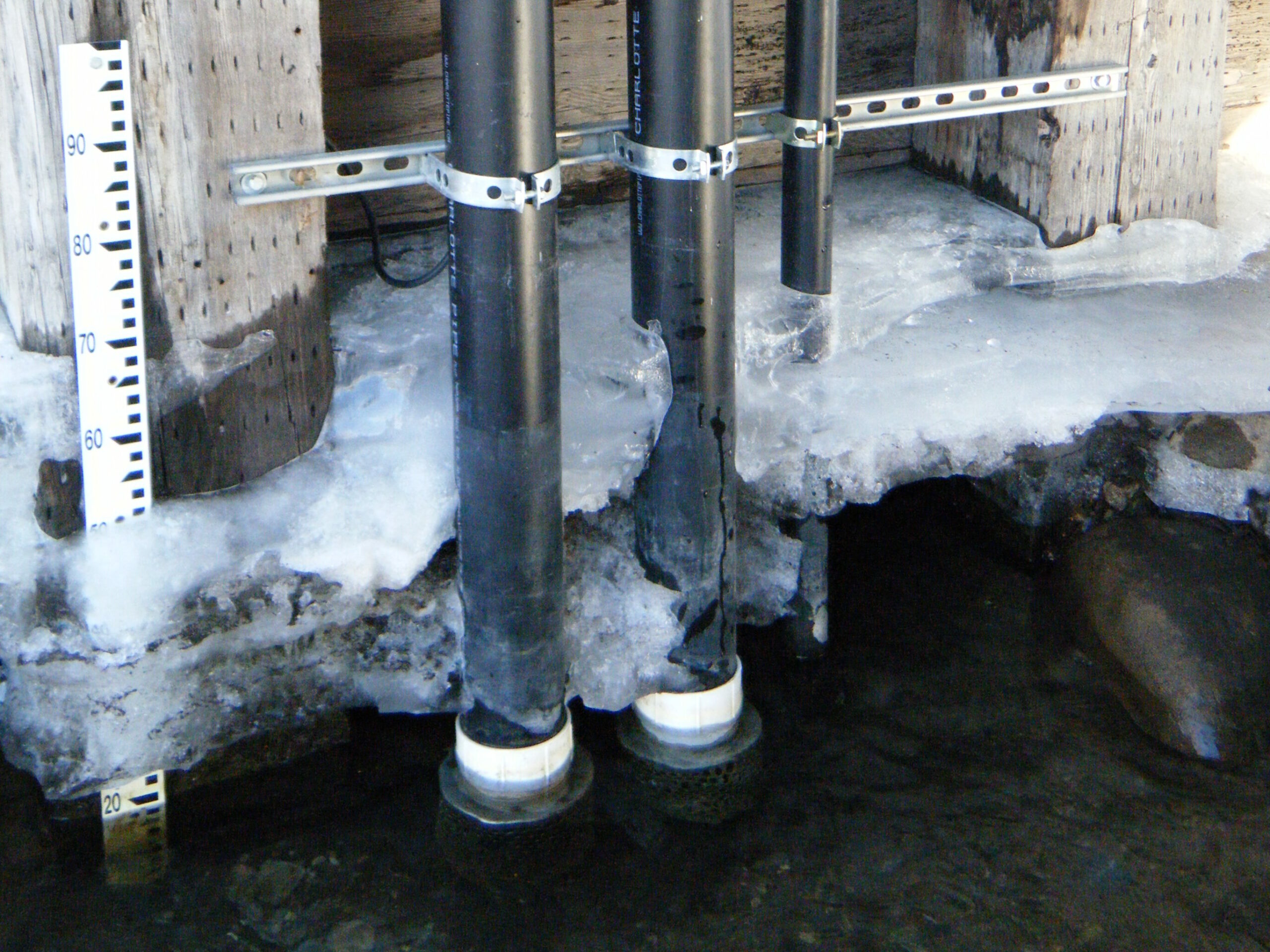
I have extensive experience with a mostly manual approach to environmental data quality control. For several years, I managed a network of monitoring stations for the iUTAH project (https://iutahepscor.org, Jones et al., 2017). I deployed both meteorological (see picture above) and hydrological instrumentation at ~10 different sites and data was recorded, typically, every 15 minutes for each sensor. Thousands of data points were transmitted back to a central database for long term storage each day. The database itself did have some simple data checks used to alert me to problems, but most of the data required manual review, a process which was both tedious and time consuming. Sometimes a sensor would break and bad data would be obvious, but other times a problem would go unnoticed for weeks. For example, hydrological instrumentation would often become dirty, buried, or, in the winter, frozen under ice (see picture below). In any of these situations, the data might appear normal when in actuality, it is no longer representative of the average value for the river. This kind of problem is largely solved by frequent site visits for cleaning.
We utilized a key piece of software, ODM tools (https://github.com/ODM2/ODMToolsPython, Horsburgh et al., 2015), which consists of a graphical user interface to visualize and manipulate data. Data visualization is essential for manual data quality control, as one is guaranteed to miss problematic data simply by looking at numbers in a file. With ODM tools, time series data can be selected, flagged, and changed. Flagging, as opposed to outright removal of data, is important because a suspicious anomaly could turn out to be a significant event. The changes are also saved to a Python script so there is a record that can be reviewed later if needed. My one critique is that ODM tools must be used with an ODM2 database (http://www.odm2.org/), hence the name, and I have found ODM2 to be overly complex. Nonetheless, I have yet to run across open source software that is similar to ODM tools.
Automated QC
My colleagues and I were able to manually quality control a significant portion of the data collected by iUTAH, but automated techniques are likely mandatory for larger projects. Automated quality control of data collected by environmental instrumentation is a fairly active area of study since at least the 1980’s and is commonly implemented on meteorological monitoring networks such as the Oklahoma Mesonet (Fiebrich et al., 2010, 2020). Several sources describe common methods for automated data assessment (Fiebrich et al., 2010, Campbell et al., 2013, Durre et al., 2010, Estevez et al., 2011). These methods typically fall into these categories:
- Range Tests – Check if data value is within a plausible range.
- Behavior Tests
- Step change – Check if the rate of change between values is plausible (spiking, jumps).
- Flatlining – Data values are overly stable and unchanging.
- Consistency Tests
- Self consistency – Data is consistent between duplicate sensors or related sensors.
- Spatial consistency – Data is consistent with measurements from nearby stations.
Since every station and network of stations is different, the details of implementing the different checks will vary and data might not even be available to complete consistency tests. For example, there is no way to check if data is spatially consistent if there is only data from one location available. Some networks, by design, have duplicate instrumentation and long term climate records, enabling more reliable range and self consistency checks. Specific QC standards are still evolving (Fiebrich et al., 2020). Nonetheless, in order to give a sense for what QC tests might look like, table below gives an example of QC test thresholds from Fiebrich et al., 2010 for a few environmental variables.
| Variable | Range | Behavior |
|---|---|---|
| Air Temperature | -30C < T < 50C | -9 C/5 min < dT/dt < 6 C/5 min |
| Air Pressure | 800 hPa < P < 1050 hPa | -4 hPa/5 min < dP/dt < 5 hPa/5 min |
| Humidity | 3% < RH < 103% | -23 %/5 min < dRH/dt < 23%/5 min |
Some methods used for self consistency tests are measurement specific. For example, wind speed is usually measured in conjunction with wind direction. When the wind speed is zero, the wind direction should not be varying and conversely, when the wind direction is changing, wind speed should be above zero. Wind speed has an interesting statistical behavior that has been used for anomaly detection in the past (DeGaetano, 1997). While working at Dyacon (dyacon.com), I investigated using ratios of average and maximum wind speed to try and detect problems with wind sensor bearings, but I never settled on a particular technique.
Another interesting example of a self consistency test is in the measurement of incoming solar radiation. Because the amount of solar radiation reaching the earth is fairly consistent (https://en.wikipedia.org/wiki/Solar_constant), the surface radiation at a given location can be calculated based on geometry and time of day. Topography and the atmosphere make the calculation complex, but ignoring those factors still provides a kind of upper bound on incoming solar radiation known as “clear sky radiation” (http://www.clearskycalculator.com/). However, I have found that clouds can sometimes create conditions where the clear sky radiation is briefly exceeded.
Automated assessment of a given measurement is challenging, but it is also very challenging to deal with missing data. Environmental data typically isn’t measured continuously. Rather measurements are taken at some frequency, like once every 10 seconds. The rate at which data should be collected depends on both what is being measured and sensor characteristics (Brock and Richardson, 2001). Therefore, missing data is defined with respect to a measurement that should have taken place but did not. This can often result from an electrical or communication problem, or it might be due to removal of values that are clearly wrong. The approach to “imputing” missing data will vary by analysis goals.
When it comes to automated QC of data, missing data can make automated calculation of statistics like mean, max, and minimum challenging. For example, at Dyacon I built a web interface for displaying daily air temperature statistics calculated from 10 minute weather station observations. It is easy to calculate an average value, but how do you assess the quality of the average value when some data is missing? Does it matter if data is missing from part of the day or lots of times through out the day? Febriech et al., 2020 gives some guidelines for how hourly and daily statistics should be calculated, but I also get the impression there is still a lack of clear standards.
Part 2
In part 2 (under development) of this series, I describe how I have implemented some of these QC concepts into a Python library: EnviroDataQC. Furthermore, I demonstrate how the package can be used in an API so that anyone can automatically perform an automated check of air temperature data (api.crceanalytics.com).
References
Brock, Fred V., and Scott J. Richardson. Meteorological measurement systems. Oxford University Press, USA, 2001.
Campbell, John L., et al. “Quantity is nothing without quality: Automated QA/QC for streaming environmental sensor data.” BioScience 63.7 (2013): 574-585.
DeGaetano, Arthur T. “A quality-control routine for hourly wind observations.” Journal of Atmospheric and Oceanic Technology 14.2 (1997): 308-317.
Durre, Imke, et al. “Comprehensive automated quality assurance of daily surface observations.” Journal of Applied Meteorology and Climatology 49.8 (2010): 1615-1633.
Estévez, J., P. Gavilán, and Juan Vicente Giráldez. “Guidelines on validation procedures for meteorological data from automatic weather stations.” Journal of Hydrology 402.1-2 (2011): 144-154.
Fiebrich, Christopher A., et al. “Quality assurance procedures for mesoscale meteorological data.” Journal of Atmospheric and Oceanic Technology 27.10 (2010): 1565-1582.
Fiebrich, Christopher A., et al. “Toward the standardization of mesoscale meteorological networks.” Journal of Atmospheric and Oceanic Technology 37.11 (2020): 2033-2049.
Horsburgh, Jeffery S., et al. “Open source software for visualization and quality control of continuous hydrologic and water quality sensor data.” Environmental Modelling & Software 70 (2015): 32-44.
Jones, Amber Spackman, et al. “Designing and implementing a network for sensing water quality and hydrology across mountain to urban transitions.” JAWRA Journal of the American Water Resources Association 53.5 (2017): 1095-1120.
Jones, Amber Spackman, Jeffery S. Horsburgh, and David P. Eiriksson. “Assessing subjectivity in environmental sensor data post processing via a controlled experiment.” Ecological Informatics 46 (2018): 86-96.