
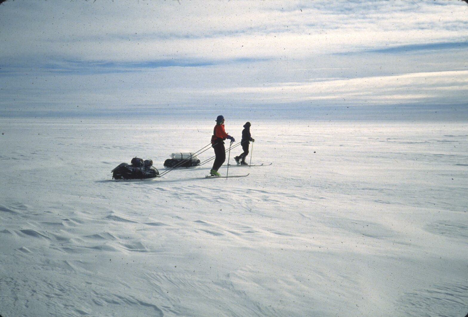
My graduate degree research was focused on glacial hydrology, which is basically trying to figure out how water moves above, below, and through glaciers and ice sheets. Water is important because it affects things like sliding, melting, sub-glacial erosion, and geochemistry. My research utilized temperature measurements from snow on the Greenland ice sheet, and I was lucky enough to travel to SW Greenland in the summer of 2010.
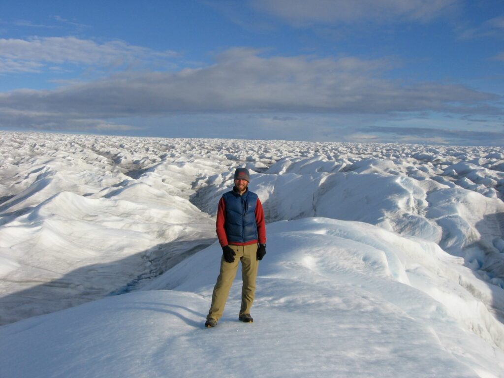
The Greenland ice sheet is about the size of the western US and is roughly 2 miles thick in the middle (promice.dk). Our work in 2010 took place on the ice surface near the margin. This area is characterized by a hummocky, rough textured surface with copious amounts of melt water streams and occasional crevasses (figure 1). We used a hot water drill to punch holes through the ~100m thick ice. The holes gave us access to perform various hydrological experiments. I attempted to trace dye beneath the ice, but ultimately had too many equipment failures to come back with usable data. I was disappointed, but had a good time nonetheless.
For my thesis, I switched gears from dye tracing to assessing snow temperature data collected from higher on the ice sheet several years before. In addition to a thesis, I eventually published a journal article on the work. Rather than let these papers be permanently frozen in academia, I want to present some of it here and if someone you find it interesting check out the links:
- Master’s Thesis:
- The Cryosphere Article:
Snow Temperature Data:
In 2007, my advisor, Neil Humphrey, and a number of other colleagues/grad students embedded an array of temperature sensors into the first 10 meters of snow pack at several different sites (figure 2). In contrast to the lumpy, stream covered ice topography of the ice margin where I did field work (figure 1), the area where the sensors were buried looks more like an endless plain of snow. This part of the ice sheet is known as the accumulation zone, where snow piles up but never completely melts. Mass is continually added to the ice sheet in this area, and what starts as snow is eventually converted, via compaction, melting and refreezing, into ice which is buried and flows down and out from the middle of the ice sheet toward the edges where it finally melts and/or falls into the sea. The sensors recorded temperatures for upwards of a year at each location, and the details documented here: Harper 2010.
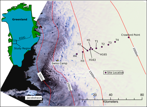
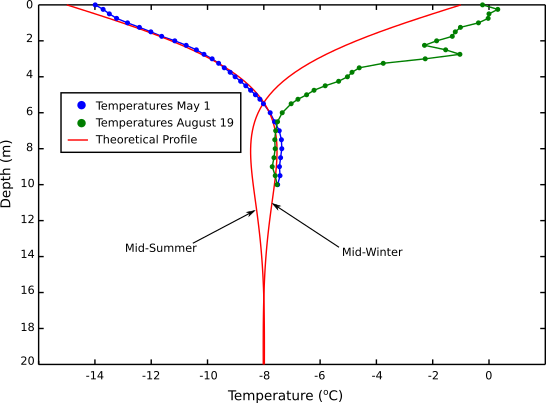
Figure 3 shows two temperature profiles from the same site: one in the late spring and one in the late summer. As one might expect, the summer profile shows higher near surface temperatures than the winter profile. Deeper down both temperature profiles converge at a temperature that is somewhat similar to the mean annual temperature for that particular site. Qualitatively, heat from the sun is conducted into the snow in summer (on average) warming the upper snow pack. In the winter that heat is then conducted back out of the snow pack, cooling it substantially. On an annual time scale, the heat going into the first 10 meters of snow roughly balances the heat going out, and the deeper temperatures remain unchanged. Interestingly, the longer the timescale the deeper the effect. So, climatological variations in temperature on multi-decadal timescales are potentially recorded in the ice profile, enabling reconstruction of past climates using ice temperature data (Cuffey and Patterson 2010). In reality, ice deformation creates added complexity, so reconstructing climate from temperature profiles has really only been attempted using boreholes drilled into the ground.
Heat Conduction Theory
Heat conduction can be modeled using Fourier’s Law, which in one dimension is:
$$ q = -K\frac{dT}{dx} $$
One dimension means that the heat is only moving in one direction, which is reasonable in certain situations such as along a narrow rod or, as I argue below, snow. Fourier’s Law states that heat flux (the amount of energy, measured in Joules, transferred through a region) is proportional to the temperature gradient at that point. So, if the temperature changes rapidly with space, heat will also be transferred at a higher rate. K is the thermal conductivity, and is a property of the material the heat is moving through. Snow has a relatively low thermal conductivity which makes it a good insulator. Note that Fourier’s Law is identical to Fick’s Law for diffusion, as heat conduction and diffusion behave exactly the same way. Other diffusive processes include groundwater flow (Darcy’s law), some types of hill slope evolution, and electrical current flow (Ohm’s law).
If you want to know what the temperature will be at a given location and time, Fourier’s Law can be used to derive the Heat Equation:
$$ \frac{\partial T}{\partial t} = k \frac{\partial^2 T}{\partial x^2} $$
While the heat equation looks complicated if you are not familiar with calculus, all it really says is that the change in temperature (T) at a location (x) is proportional to the curvature (temperature spike = high curvature) of temperature at that location. The heat equation can be solved for certain well defined situations resulting in a function that describes how the temperature varies with time (t) and location: T(t,x)
Although snow pack is a three dimensional structure with a high degree of variability in density and ice crystal shape and bonding, it is reasonable to approximate it as one dimensional for some problems. In this case, we are assessing how snow temperatures change with depth at the scale of several centimeters, and there are several reasons why a one dimensional approach may be appropriate. First, if refreezing of water is ignored, any large changes in temperature occur at the upper surface driven by changes in solar radiation and air temperature. In Greenland, where the surface doesn’t change all that much over long distances, the surface heating/cooling is relatively uniform and therefore the temperature at the surface should be relatively uniform. This means that heat won’t really be moving sideways, just up and down. Second, although at small scales ice crystals can be highly variable with different shapes and degrees of bonding, these small scale variations “average out” and the snow can be thought of as a continuous mass with a particular thermal conductivity rather than a bunch of particles. Finally, since snow is building up from above, any variations in density that affect how heat is conducted are mostly the vertical direction.
If you are willing to accept approximating heat conduction in snow as being largely one dimensional, just a few more assumptions are needed to get an analytical solution to the heat equation. Ideally, one would just adapt the heat equation for a particular site using measured thermal conductivities, surface temperatures, and a starting temperature profile. Then solve the equation to get a function T(t,d) that describes what snow temperatures will be at a certain time and depth. In reality, mathematicians have only figured out how to solve the heat equation in certain situations. This forces us to simplify the problem a bit more and our final solution is based on the following:
- One dimensional heat conduction
- Thermal conductivity is constant with space and time
- Surface temperatures change according to a sin wave
- Snow pack is infinitely deep
Of those simplifications, holding thermal conductivity constant with depth is likely the least realistic. The true thermal conductivity will vary with depth depending on density and ice crystal shape. A sin wave approximation for surface temperature is reasonable because both daily and annual surface temperature changes follow a wave pattern resulting from changes in solar radiation. Furthermore, the heat equation has a property that rapid temperature changes are not conducted very far and can largely be ignored. So, a few unusually cold days are not going to have much of an affect on the temperature profile. Finally, a infinitely deep snow pack is reasonable for Greenland where the ground might be kilometers below the surface and we are only looking at the first 10 meters. It wouldn’t be a reasonable simplification in a mountain snow pack.
A solution to the heat equation with the assumptions described above takes the form:
$$ T(d,t) = A \exp(-d\sqrt{w/2k})\sin(wt – d\sqrt{w/2k}) $$ (Cuffey and Patterson 2010)
Data vs Theory
In order to actually use the solution calculated above, we need to define the frequency (w) and, amplitude (A) of the surface temperature sin wave, as well as, plug in a snow thermal conductivity. While we could come up with a sin wave using measured snow surface temperatures, I thought it would be more interesting to use a completely separate data set from the snow profile temperatures. At one of the temperature profile sites, Crawford Point, another research group (Greenland Climate Network) has a long running weather station. Using air temperature data from the weather station (air and surface temperatures are reasonably close), we can calculate theoretical temperature profiles to compare to the measured profiles. This approach has a number of benefits that I think are scientifically more rigorous. Using separate datasets ensures that the calculated profiles are not biased toward the measured profiles. It is vaguely circular to calculate temperature profiles from measured data and then compare the results to those same measurements. The measured surface temperatures in the temperature profiles are also highly suspect. Surface melting, accumulations, and solar radiation warming the sensor directly all contribute to increased uncertainty/bias in near surface temperature measurements.
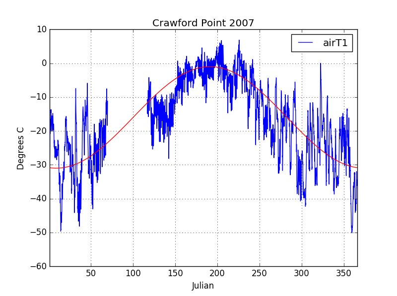
In figure 4, I plotted a “best fit” (just eyeballed) sin wave to air temperature data from 2007. Note that the average temperature is around -15C and that the air temperatures only reach near freezing mid summer – ice sheets are cold! The equation of this sin wave is:
$$ T(t) = 15\sin(\frac{2\pi}{365}(t+100)) – 16 $$
For thermal conductivity we can use a value computed as a function of density. Density and thermal conductivity are not perfectly correlated, but density is easy to measure and, for higher density snow packs like those found in Greenland, there is less variation in thermal conductivity than for lower densities (Sturm et al., 2007). The relationship between density and thermal conductivity was another component of my thesis, and maybe I will do another blog post on it someday, but for now I will just use a thermal conductivity value of 1.5 (W/mK) given a snow density of 700 (kg/m^3).
Putting it all together our final equation for a theoretical temperature profile is:
$$ T(d,t) = 15 \exp(-d\sqrt{w/2k})\sin(w(t+100) – d\sqrt{w/2k}) – 16 $$
Diffusivity (k) is calculated from conductivity using a snow density of 700 (kg/m^3) and a specific heat capacity of 2097 (J/kg*K). Note that there are also some unit changes involving seconds to days.
Analysis
Unfortunately, the snow profile data from Crawford Point is limited to late June thru October 2007, so we cannot compare mid winter profiles. Nonetheless, figure 5 shows three comparison plots from the beginning, middle, and end of the data set. In general, the match between theory and data is by no means perfect, but does reflect the general shape of the data. In both theory and data, the 10m temperature is relatively stable with time and is very similar to the mean annual air temperature. Both curves show a subtle pattern of a temperature wave that travels from the surface into the snow pack over the course of the four month period. To put it another way, the increase and decrease in temperatures in the near surface over the summer is also present in the lower profile, but it occurs later and has a smaller magnitude.
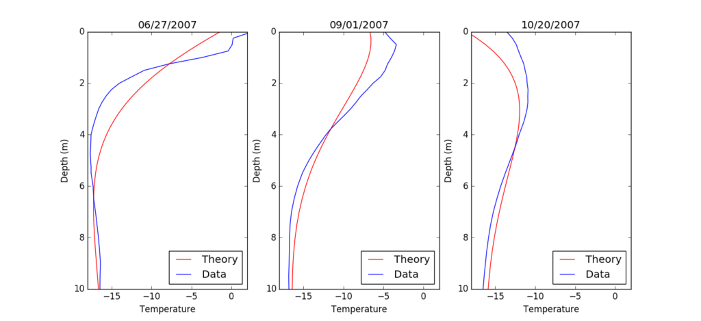
One feature that does stand out is the top 1m of snow in 6/27/2007. Here there is a sharp bend in the data and even above zero temperature readings. Surface melting in this area has likely exposed the top one or two temperature sensors to solar radiation which heats the sensor itself above that of the underlying snow. Regardless, at each point in time, the observed temperatures in the near surface snow are higher than predicted by theory. The explanation for this is something I mentioned briefly earlier: melt water refreezing. In the summer, the surface melt soaks into the cold underlying snow and refreezes. The refreezing releases heat and warms the surrounding snow pack until it eventually reaches 0 C, as is seen in the data from 6/27/2007.
Melt water infiltration and refreezing is much more significant of a phenomenon than one might expect. The melt water can form vertical channels and penetrate into the snow pack much deeper than is possible with uniform infiltration. Recent research (Nature Paper) has also found that, in some areas, melt water can form aquifers in the snow that remain liquid year round. Knowing how much melt water is stored in the snow and how much runs off is important for determining if the ice sheet is growing or shrinking.
References
Paterson, W.S.B, The physics of glaciers, Academic Press, 3rd Ed, 2010.
Sturm, M., Holmgren, J., Konig, M., Morris, K., The thermal conductivity of seasonal snow, Journal of Glaciology, Vol. 43, No.143, 1997.