I wrote this a few years ago on another blog, but I think it is still relevant so I am re-posting it here. The code is still available on Github.
I worked for several years at USU on the iUTAH project. While there I managed a network of water monitoring stations along the Logan river, and one component of my job involved measuring stream flow. We wanted to know how much water was flowing past each station in order to answer basic questions like “how much water is lost or gained downstream?”
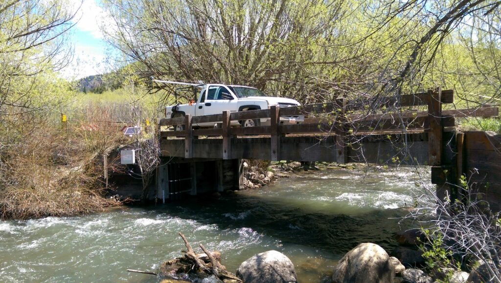
It is amazing how much Earth Science is simply trying to figure out how much of a particular thing there is in a particular spot. How much water is there? How deep is the snow? How much precipitation falls on the ground? In the case of stream flow, also known as discharge, things get a little tricky because fluid mechanics is complex. For example, water near the surface moves downhill faster than water near the stream bed due to friction. Furthermore, the flow is highly turbulent, so there are lots of eddies and waves. If the water is channeled through an engineered structure with a specific geometry, the flow can be calculated, but a natural river channel has an irregular shape that changes through time. In this situation the typical approach is to make lots of measurements across the channel and add them all together to get a total flow. While various instruments with different degrees of accuracy have been invented to make these measurements, sometimes ones only option is to hang a water velocity meter from a truck with a big weight (see figure 1).
I won’t detail the various methods used to measure discharge in this post. Rather, my goal here is to present a tool for performing a regression on discharge measurements against the elevation of the water surface, also known as stage. Relating stage to discharge (a “rating curve”) enables you to take something that is easy to measure, water depth, and convert it to something that is difficult to measure, flow. In general, measurement of stream flow is a huge component of hydrology and I don’t claim to be an expert. The analysis presented here mostly follows Herschy 2008. But, I do think there is a need for more open source calculation tools, so I hope the python code discussed below is helpful for a working hydrologist, student, or researcher.
Rating Curve Theory
While I expect someone who is interested in using the rating curve notebook to have a little bit of knowledge of open channel hydrology, I also think it is helpful to give a bit of an overview of the theory because it is needed to properly use the notebook.
A rating curve is simply a regression relating stage and discharge. The classic approach is to fit the data with an equation of the form:
$$ Q(h) = C(h-a)^{\alpha} $$
Q = discharge (cms), h = stage (m), and a = effective height of zero flow (m).
C and alpha are parameters derived from the regression, and as discussed below, the value of alpha may give some insight into the factors influencing the relationship between stage and discharge. This equation is generally described as a “power law” because the dependent variable is related to the independent variable by some power. Power law functions are very common in physics and earth science. There is probably some deeper reason for it, but I don’t know what it is off the top of my head. Aside from the commonality of this type of equation, there is some additional logic behind using a power law over some other curve. After all, one can fit any curve to any data. In this case, the power law relationship is used because it has the same form as the “manning equation”.
$$ Q = \frac{K}{n} * h^{5/3} * slope ^{1/2} * width $$
This is basically $Q=Constants*h^{5/3}$ which is only different in that it lacks ‘a’. The Manning equation is derived via a conservation of energy analysis of flow in a rectangular shaped channel (Hornberger et al. 1998). The equation components are basically just the driving and resisting forces acting on the water: gravity (slope) and friction. In this equation, alpha = 5/3, but a natural channel is rarely rectangular, so one wouldn’t expect it to be exactly 5/3 as determined by regression.
Thus far I neglected to discuss parameter ‘a’, the effective height of zero flow, because it will make more sense after a short discussion on “controls”. Different sites will most likely have different rating curves (values of C and alpha) because each site has a different (a least slightly) set of characteristics that influence the flow including channel shape, bank vegetation, meanders, and constrictions (Herschy 2008). These characteristics are known as a “control” since they control the shape of the rating curve. A control can be broadly classified into two groups: section and channel. A section control is a localized somewhat specific feature that has a big influence on flow regardless of what is going on downstream. A waterfall a short distance downstream from a station is one example of a section control because it will be the main feature influencing how flow varies with water depth regardless of what is going on downstream. A channel control exists when the rating curve is determined by the collective effects of all the site characteristics as a whole rather than a specific feature.
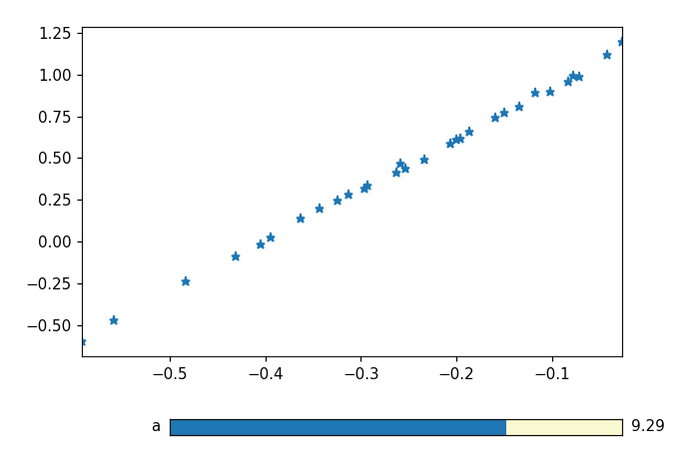
Going back to parameter ‘a’: In the Manning equation the discharge is a function of the depth of the flow, but in an irregularly shaped natural channel the depth is variable across the cross-section. Instead of using depth of flow, the regression is based on the depth of flow above the elevation of zero flow. Intuitively, zero flow might be the elevation of the bottom of the channel, but often it is not, especially for a section control. If a section control is behaving somewhat like a dam, the depth of zero flow would be the lip of the dam, not the depth of the pool. Furthermore, at higher flows a localized feature might be completely submerged and the “effective” elevation of zero flow corresponding to the high flow channel control might not be different from lower flow value of ‘a’. In that situation, there might be two different rating curves representing the overall river behavior. While ‘a’ can be estimated in the field, the easiest approach to determining ‘a’ is to plot the stage-discharge measurements in log-log space. Using a trial and error procedure, ‘a’ can be estimated by adjusting the value of ‘a’ until the stage-discharge values plot in a straight line (see below).
Jupyter Notebook
Now, an overview of the the Jupyter Notebook Template. The template is available on Github along with some data one can use to give it a try. I assume you have some experience with Python and the Jupyter project. Input data consists of discharge measurements and associated stage readings for a particular site. The final “output” at the end of the template is an equation of the form $Q = C(h-a)^{\alpha}$. Each cell in the notebook is described to some extent, but I will elaborate on a few items below. Some cells are blank leaving room for analysis and interpretation of data from a particular site enabling one to share how a particular rating curve came to be.
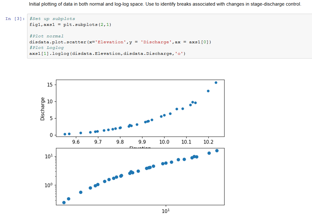
An initial plot of the stage-discharge data is created in both “linear” and log-log space. The linear plot can help identify outliers or odd features in the data. The log-log can be used to identify any major changes in the slope of the data. This could signify that the control changes substantially at a particular flow and it might be best to construct two separate rating curves rather than one.
The effective height of zero flow should be somewhat similar to the thalweg of the river, but will vary somewhat depending on the nature of the control at the site. At a station with an obvious section control, the height of zero flow can be estimated from height measurements of the base of the control. However, it may be easier to use a graphical approach to estimating ‘a’. A reasonable value for ‘a’ will result in a more linear plot of the stage-discharge points while bad values of ‘a’ will result in the plotted points showing some curvature. Depending on the amount of scatter in the measurements, the best value for ‘a’ may remain unclear so it is important to verify the final value is realistic. The notebook has a slider for adjusting the value of ‘a’ between the minimum measured stage value and that value minus 1m.
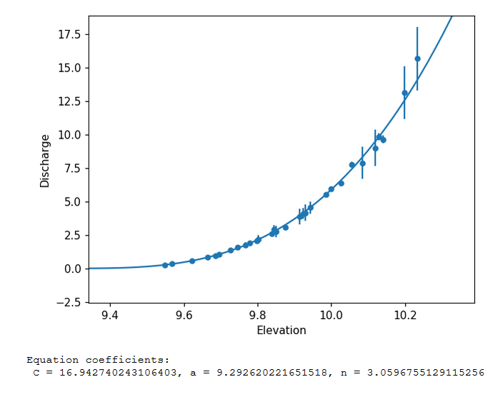
The final step in the process is simply performing a standard linear regression on the data. It would be nice if error in measurement could somehow be included in the regression with higher accuracy measurements being weighted more than lower accuracy measurements. Unfortunately in my literature search, I didn’t see any obviously simple approaches to that problem. The final plot in the notebook shows the points as well as the rating curve and the regression parameters.
References
Herschy, R. W., 2008, Streamflow measurement. CRC press.
Hornberger, G.M., Raffensperger, J.P., Wiberg, P.L., Eshleman, K.N., 1998, Elements of Physical Hydrology, John Hopkins University Press.